Black-Scholes Model
There are three basic types of information that are relevant to the default probability of a publicly
traded firm: financial statements, market prices of the firm's debt and equity, and subjective appraisals of the
firm's prospects and risk.Prices,by their nature, are inherently forward looking.In determining market
prices, investors use,amongst many other things,subjective appraisals of the firm's prospects and risk,
financial statements and other market prices.This information is combined using their own analysis and
synthesis and results in their willingness to buy and sell the debt and equity securities of the firm.
Market prices are the result of the combined willingness of many investors to buy and sell and thus prices
embody the synthesized views and forecasts of many investors.
Merton's general derivative pricing model was the genesis for understanding the link between the market
value of the firm's assets and the market value of its equity.We use the Black-Scholes option pricing
model as a special case of Merton's model,to illustrate some of the technical details of estimating
EDF values.Here, I work the calculation of an EDF value using the BS option-pricing model.
Equity has a residual claim on the assets after all the obligations have been met.It also has limited
liability.A call option on the underlying assets has a claim on the assets after meeting the strike price
of the option.In this case the strike of the call option is equal to the book value of the firm's libilities.
If the value of the assets is insufficient to meet the liabilities of the firm then the shareholders,
holders of the call option will not exercise their option and leave the firm to its creditors.
We exploit the option nature of equity to derive the market value and volatility of the firm's
underlying assets implied by the equity's market value.In particular, we solve backwards from the
option price volatility for the imlplied asset value and asset volatility.
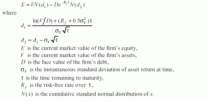
The Black-Scholes formula gives the value of equity today as:

The risk-neutral probability that the company will default on the debt is N(-d2).To calculate
this, we require V and  . Neither of these are directly observable.However if the company is publicly
traded we can observe E.This means that the above equation provides one condition that must be satisfied by
V and
  . We can also estimate
  . From Ito's lemma,

This provides another equation that must be satisfied by V and  . The above 2 equations can be solved
simultaneously for V and
  .
.
Due to the arbitrary complexity of solving the above two equations for a large number of firms , I use
the book-value-implied asset volatility instead of the above equity-implied asset volatility given
by Ito's lemma.The book-value-implied asset volatility is as follows:

Recall also,that the distance to default is the number of standard deviations that the firm is away from
default and thus in the BS world is given by d2.
Estimating equity/asset volatility from Historical Data
Volatility is measured as the standard deviation of the returned provided by the equity/asset in one year
when the return is expressed using continuous compounding. Using the lognormal property of stock/equity values
volatility is calculated as follows:
Compute S(t)/S(t-1), where S(t) is quarter t equity value
Compute u(t)= ln[S(t)/S(t-1)]
Find the Standard Deviation of u(t).This estimates the quarterly volatility
If the volatility is v for one unit of time the volatility for t units of time is vt1/2.Thus we go from
quarterly to annual volatility by multiplying by 2.
The only problem in implementing remains in calculating the cumulative normal distribution function,N.
A polynomial approximation that gives six-decimal-place accuracy is as follows(See M.Abramowitz and I.Stegun,
'Handbook of Mathematical Functions,Dover Publications,New York,1972):

Results
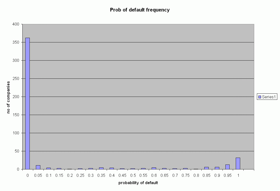
Click here to see the probability of default for the S&P 500 publicly traded companies.
Click here for the code.


 . Neither of these are directly observable.However if the company is publicly
traded we can observe E.This means that the above equation provides one condition that must be satisfied by
V and
  . We can also estimate
  . From Ito's lemma,

 . The above 2 equations can be solved
simultaneously for V and
  .
.


